Attention is a useful and versatile tool used in various deep learning approaches. In this post, we will look into the main concepts behind attention and its use in the Transformer model.
- Motivation
- Origin of The Attention Mechanism
- Formal Definition
- Variations of Attention Mechanism
- Transformer
- References
Motivation
Attention mechanism in the topic of learning algorithms is motivated by how we, humans, pay attention to different components of our sensory inputs. In the context of visual attention, depending on our objective, we bring different components of our visual input to focus and blur the rest (Hoffman and Subramaniam, January 1995). Figure 1 (a) shows an image of maple taffies with a patch of the image masked. If we were to guess the content of the masked region, we would pay more attention to certain areas of the image, while ignoring the rest. The pink areas shown in Figure 1 (b), depicting the twisted fingers holding a popsicle stick, some maple syrup on the snow, and a popsicle stick attached to the maple syrup, will lead us to guess that the masked region must be covering a rolled up maple taffy. Other regions in Figure 1 (b) such as the background, or the color of the person’s sleeve (indicated by gray circles) do not contribute to our decision-making.
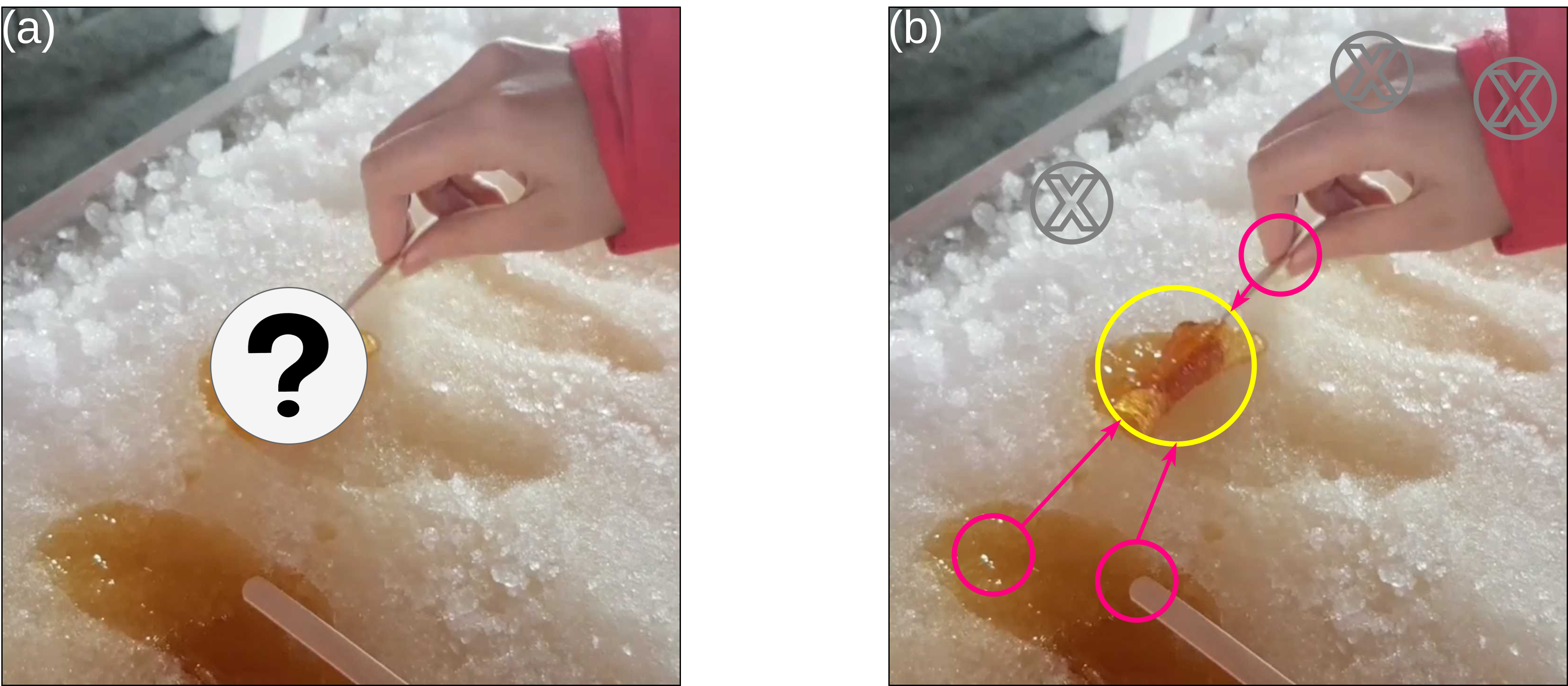
Figure 1: (a) Masked image (b) Attention to the pink circles help guess the content of the masked region, while the gray regions receive no attention.
In the context of natural languages, we perceive similar contextual correlation between different components. For example in the sentence:
I drank a glass of water.
We expect a liquid to appear in the sentence once we read the word drank. There is a strong correlation between these two words in this sentence. Hence, as shown in Figure 2, the word drank attends to the word water, however it does not directly attend to the word glass.
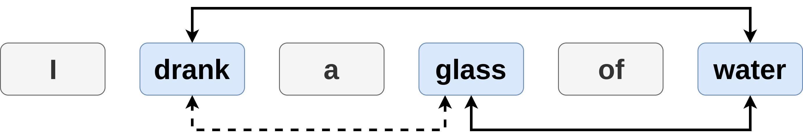
Figure 2: Solid arrows indicate high attention. Dashed arrow indicates low attention.
In the context of learning algorithms, attention is a mechanism distributes importance weights to the components of an input (e.g. pixels in the image domain and words in natural languages) in order to infer a target output. These importance weights indicate the correlation between the input components, and the target outputs. In other words they specify how strong the algorithm should attend to different components of the input to infer the target outputs.
Origin of The Attention Mechanism
In order to better understand the importance and advantages of the attention mechanism, we first need to look at the problem it tries to solve. For this purpose, we briefly examine the sequence to sequence model architecture.
The sequence to sequence model or encoding-decoding architecture is an extension of the RNN. It is the standard model architecture for many NLP tasks such as: language modeling (Sutskever et al., December 2014), neural machine translation (Bahdanau et al., May 2015; Cho et al., October 2014), and syntactic constituency parsing (Vinyals et al., December 2015). This architecture, transforms an input or source sequence to an output or target sequence. These sequences can be of arbitrary length and not necessarily equal to each other. The architecture of sequence to sequence model is composed of: an encoder mechanism and a decoder mechanism.
The encoder operates on the source sentence, and compresses it to a fixed length vector known as the context vector or sentence embedding. The context vector is expected to be a rich representation of the source sentence containing a sufficient summary of the source information. A classical choice for the context vector is the last hidden state of the encoder (Cho et al., October 2014). The decoder constructs the target sentence based on the context vector it receives from the encoder. Both encoder and decoder architectures are based on RNNs i.e. using LSTM or GRU units. Figure 3 shows the encoder-decoder model used in neural machine translation for the following translation:
English: Watermelon is delicious.
French: La pastèque est délicieuse.
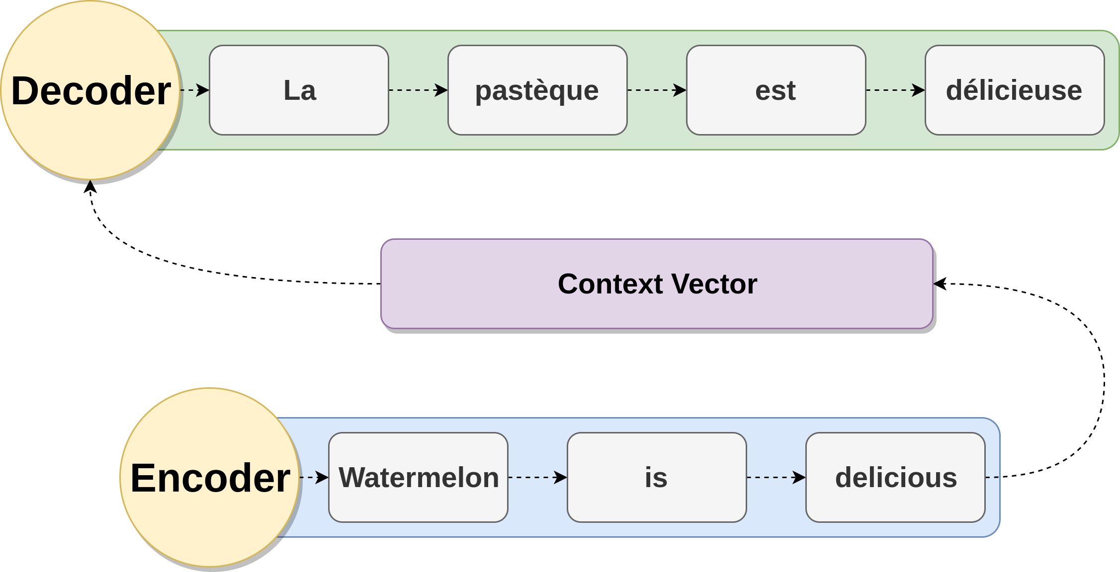
Figure 3: Encoder-decoder architecture used in neural machine translation, translating the sentence «Watermelon is delicious» to French.
Bahdanau et al. (May 2015) showed that a major drawback of using fixed-size context vectors is the limitation of this vector to summarize and remember all the necessary information in the source sentence. Having a fixed-size context vector introduced a bottleneck on the performance of sequence to sequence models. When the model is presented with longer length source sentences, the model would simply forget part of the information from the earlier part of the source sentence. In the context of neural machine translation, this led to poor and incoherent translations for longer sentences (Bahdanau et al., May 2015). Attention mechanism was, therefore, proposed by Bahdanau et al. (May 2015) to remedy this issue.
In the context of Neural Machine Translation (NMT), Attention mechanism helps the encoder-decoder network memorize longer length source sentences. Attention mechanism allows the context vector to create links between the entire hidden representations of the source sentence, instead of using a single fixed sized context vector from the last hidden state of the encoder. These links are parameters learned by the network, and they are adjusted for each output element in the target sequence. Since the context vector has access to the entire source sentence, the performance of the encoder-decoder network is not affected by the length of the source sentences. Figure 4 shows the encoder-decoder model augmented with an attention mechanism to construct dynamic context vectors.
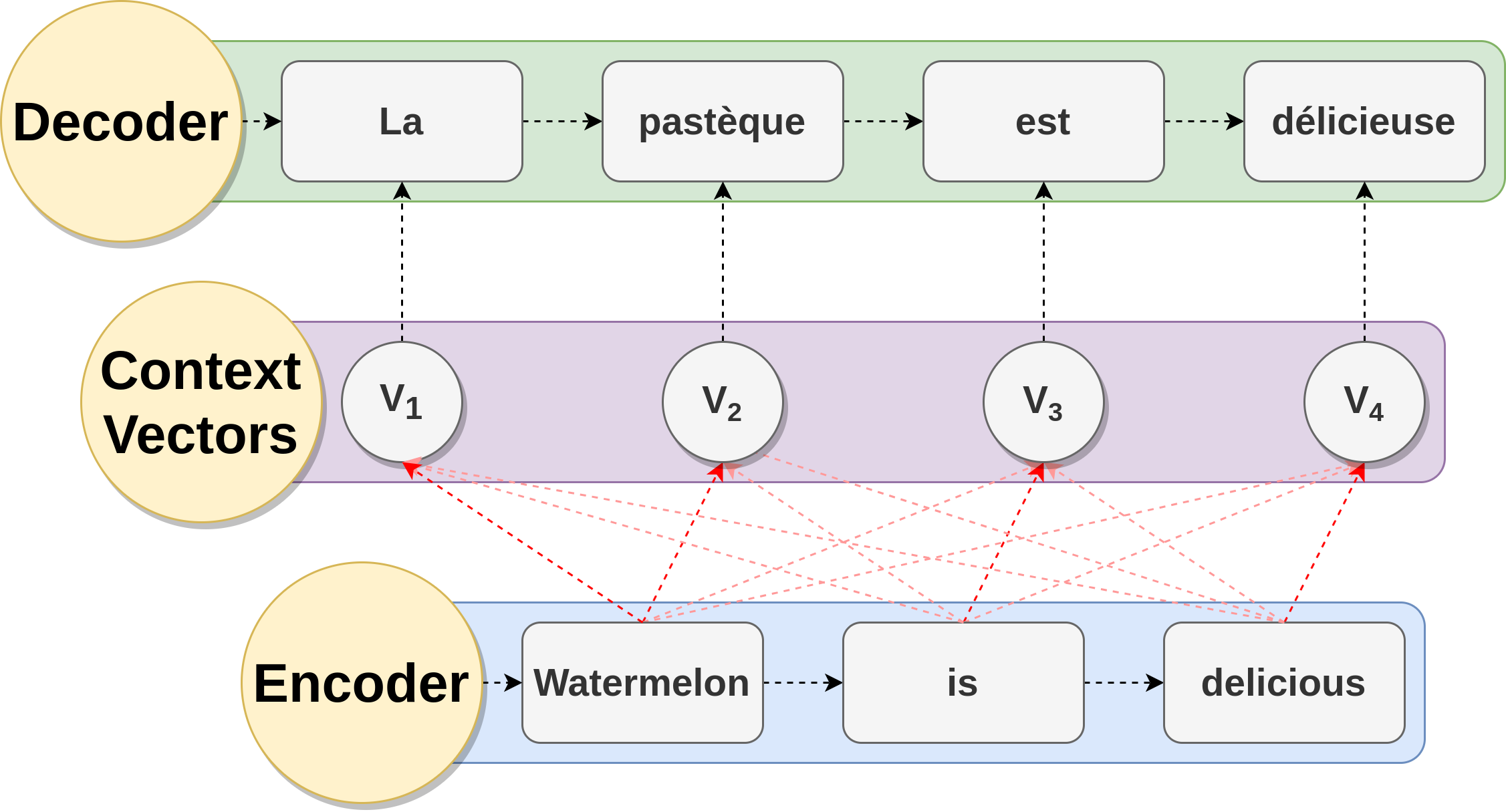
Figure 4: Encoder-decoder architecture augmented with attention mechanism used in neural machine translation, translating the sentence «Watermelon is delicious» to French. Bright red arrows indicate higher attention values.
Formal Definition
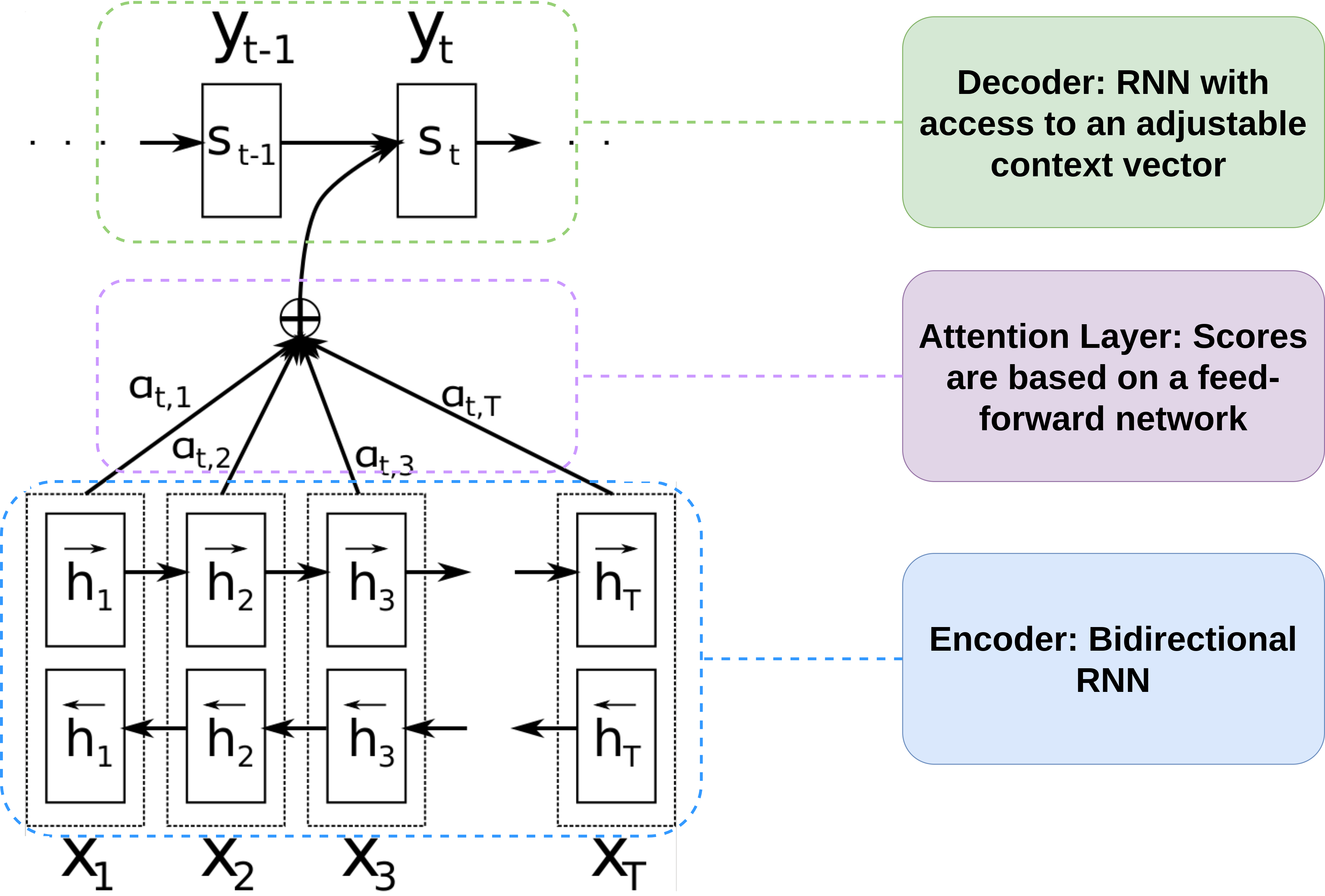
Figure 5: Neural machine translation architecture used by Bahdanau et al. (May 2015).
Since the attention mechanism was introduced in NMT, we will base the examples of this section on this task, and we will focus on the encoder-decoder architecture that was proposed by Bahdanauet al. (May 2015). Assume, that we have a source sequence \(x\) of length \(T\), and the target sequence \(y\) of length \(M\):
\[x = \left[x_1, x_2, \dots, x_T \right] \\ y = \left[y_1, y_2, \dots, y_M \right]\]The encoder will receive the source sequence \(x\) and will produce hidden state representations \(h_i\) at time step \(i\). As shown in Figure 5, in the architecture proposed by Bahdanau et al. (May 2015) the encoder is a bidirectional RNN and \(h\) at time \(i\) is defined as:
\[h_i = \left[\overrightarrow{h_i},\overleftarrow{h_i}\right] \hspace{0.2cm} \forall i \in \{1,2,\dots,T \}\]Where \(\overrightarrow{h_i}\) is the hidden state representations in the forward pass of the RNN and \(\overleftarrow{h_i}\) is the hidden state representations in the backward pass of the RNN. The decoder will produce hidden state representations \(s_j\) defined for time \(j\) as:
\[s_j = f(s_{j-1},y_{j-1},c_j) \hspace{0.2cm} \forall i \in \{1,2,\dots,M \}\]Where \(f\) computes the current hidden state given the previous hidden state, the previous output, and the context vector. \(f\) can be either a vanilla RNN unit, a GRU, or an LSTM unit. The parameter \(c_j\) is the context vector at time \(j\) computed as a weighted sum of the source sequence hidden representations:
\[c_j = \sum_{i=1}^{T} \alpha_{ji}h_i\]Where the weights \(\alpha_{ji}\) for each source sequence hidden state representation, \(h_i\), are alignment measures indicating how well an input at position \(i\), and an output at position \(j\) match:
\[\alpha_{ji} = \mathrm{align}(y_j,x_i)\]The alignment measure is a probability distribution over a predefined alignment score function. The score for the input at position \(i\) and output at position \(j\) is computed based on the hidden representation of the input at position \(i\), \(h_i\), and the hidden representation of the decoder at position \(j-1\), right before emitting the output \(y_i\):
\[\mathrm{align}(y_j,x_i) = \frac{ \exp{ \left( \mathrm{score}(s_{j-1},h_{i}) \right) } } { \sum_{r=1}^{T} \exp{ \left( \mathrm{score}(s_{j-1},h_{r}) \right) } }\]In the architecture proposed by Bahdanau et al. (May 2015) a feed-forward neural network is used to parametrize and learn the alignment scores. The feed-forward network is composed of a single hidden layer with \(\tanh\) activation function and is jointly trained with the other parts of the network. Hence, the alignment scores are given by:
\[\mathrm{score}(s_{j},h_{i}) = v \hspace{0.1cm} \mathrm{tanh}\left( W [s_j,h_i] \right)\]Where \(v\) and \(W\) are weight matrices that will be learned by the network. These alignment scores define how much of each of the source hidden states is needed to produce each of the target outputs or in other words, how much the target words should attend to the source sequence in the decoding process. This concept is captured by the matrix of the alignment scores, explicitly showing the correlation between input and output words. Figure 6, shows the matrix of alignment scores for an English-French translation.
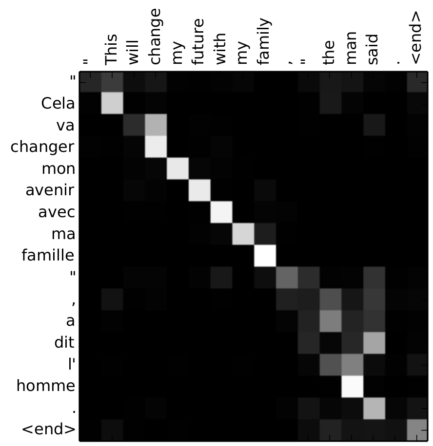
Figure 6: Matrix of alignment scores for the translation of «“This will change my future with my family,” the man said.» to French, «“Cela va changer mon avenir avec ma famille”, a dit l’homme.» Figure is taken from Bahdanau et al. (May 2015)
Variations of Attention Mechanism
Success of the attention mechanism in NMT motivated researchers to use it in different domains (e.g. computer vision (Xu et al., July 2015)) and experiment with various forms of this mechanism (Vaswani et al., January 2017; Luong et al., September 2015; Britz et al., September 2017). The first natural extension to this mechanism is the alignment score function.
As discussed in previously, Bahdanau et al. (May 2015) used a single feed-forward neural network with a \(\tanh\) activation function to compute the alignment scores. However, other approaches have been proposed for the alignment score function. Table 1, lists a few popular alignment score functions.
| Name | Alignment Score Function | Used In |
|---|---|---|
| Content-based | \(\mathrm{score}(s_j , h_i) = \cos(s_j, h_i)\) | Graves et al. (December 2014) |
| Additive | \(\mathrm{score}(s_j , h_i) = v \mathrm{tanh}\left( W [s_j,h_i] \right)\) | Bahdanau et al. (May 2015) |
| Dot Product | \(\mathrm{score}(s_j , h_i) = s_j^T h_i\) | Luong et al. (September 2015) |
| General | \(\mathrm{score}(s_j , h_i) = s_j^T W h_i\) | Luong et al. (September 2015) |
| Location-base | \(\mathrm{score}(s_j , h_i) = W h_i\) | Luong et al. (September 2015) |
| Scaled dot product | \(\mathrm{score}(s_j , h_i) = \frac{s_j^T h_i}{\Vert h_i \Vert}\) | Vaswani et al. (January 2017) |
Table 1: Popular Alignment Score Functions for an Attention Mechanism.
Aimed to reduce the computation costs of attention mechanism, Xu et al. (July 2015) experimented with two kinds of attention mechanism: soft attention and hard attention. Soft attention is similar to the attention mechanism introduced by Bahdanau et al. (May 2015) as it assigns a (soft) probability distribution to all the source hidden states, which makes the model smooth and differential but costly in the computation time.
On the other hand, hard attention aims to reduce the computation cost of attention mechanisms by only focusing on one single source hidden representation at a time. The attention mechanism in this setting is representing a multinoulli probability distribution over all the source hidden states. Therefore, the vector of the attention weights is a one-hot vector assigning a weight of 1 to the most relevant source hidden state and 0 to the others.
The one-hot representation of the attention is non-differentiable hence it requires more complicated techniques such as variance reduction or reinforcement learning to train (Luong et al., September 2015). In order to remedy the non-differentiability of hard attention, Luong et al. (September 2015) proposed the concept of local attention. In their work, they call the soft attention mechanism, the global attention since it attends to all hidden states in the source sequence. The local attention, on the other hand, only attends to a window of the source hidden states. This mechanism first predicts a single aligned position for the current target word mimicking the behavior of the hard attention. A window centered around the source position is then used to compute the context vector similar to the mechanism of soft attention. The local attention mechanism perfectly blends soft and hard attention together to save computation costs while preserving the differentiability of the model.
Self-attention or intra-attention is a special case of the attention mechanism where the source and target sequence are the same sequence. The context vector formulation is the same as before, however, the weights are formulated differently. As a result, the target sequence is replaced by the source sequence leading to:
\[\alpha_{ji} = \mathrm{align}(x_j,x_i)\]The attention mechanism in this setting will find the best correlation between each word in a sentence and the others, making self-attention an integral part of the recent advancements in embedding representations (Vaswani et al., January 2017; Devlin et al., June 2019; Yang et al., June 2019).
Transformer
RNNs have been the preferred building block for time series data. Due to their ability of processing sequential inputs of variable length and capturing the sequential dependency of the data, these architectures have been the preferred building block for many NLP neural approaches such as language modeling (Sutskever et al., December 2014), neural machine translation (Bahdanau et al., May 2015; Cho et al., October 2014), and syntactic constituency parsing (Vinyals et al., December 2015). However, RNNs are only slightly parallelizable, that means the computational resources cannot be fully utilized during training and hence, leading to a very time-consuming training process.
In order to mitigate this issue, Vaswani et al. (January 2017) proposed the Transformer architecture. The Transformer model is solely based on the attention mechanism and uses self attention layers to learn word representations. In the context of sequential data, the Transformer architecture is superior to the classical neural architecture approaches such as RNNs or CNNs based on three important criteria: computation complexity, parallelizability, and long-term dependency modeling.
The computation complexity of the Transformer model is \(O(n^2.d)\) for a sequence of length \(n\) and hidden representation of size \(d\), as opposed to RNNs and CNNs which have a computation complexity of \(O(n.d^2)\) and \(O(k.n.d^2)\) respectively, where \(k\) is the kernel size of the convolution. The dominating factor determining computation complexity of the model is the dimension of the hidden representation, since it is typically far larger than the sequence length, or the kernel size. Hence, the Transformer model is conserving computation complexity by \(O(d)\) compared to the other two models.
As mentioned before, RNN computations are only slightly parallelizable, leading to a sequential computation of \(O(n)\) on a sequence of size \(n\), since the model essentially needs to loop through the sequence. However, Transformer and CNN models are highly parallelizable by design, having \(O(1)\) sequential computations.
Modeling long-term dependencies of a sequence input is a challenging task (Bengio et al., March 1994; Bahdanau et al., May 2015). The length of the path between long range dependencies has an inverse correlation with the ability of the model in learning these dependencies. Longer paths prevent the gradient or learning signals to be transmitted smoothly (Bengio et al., March 1994). Hence, the shorter the path between long range dependencies, the better the model learns. CNNs with a kernel of size \(k\) have a maximum path length of \(O(\log_k(n))\) for a sequence of size \(n\), while RNNs have a maximum path length of \(O(n)\). Since Transformers are solely based on the attention mechanism, the maximum path length in this architecture is \(O(1)\), letting the model to seamlessly capture long-term dependencies of sequential inputs. Table 2, lists a summary of computation comparison between the Transformer model, RNN, and CNN.
| Transformer | RNN | CNN | |
|---|---|---|---|
| Computation complexity | \(O(n^2.d)\) | \(O(n.d^2)\) | \(O(k.n.d^2)\) |
| Sequential computation | \(O(1)\) | \(O(n)\) | \(O(1)\) |
| Long range dependency | \(O(1)\) | \(O(n)\) | \(O(\log_k(n))\) |
Table 2: Computation comparison between the Transformer model, RNN, and CNN for a sample of size \(n\), hidden representation of \(d\), and CNN kernel size of \(k\).
Multi-Head Attention
Vaswani et al. (January 2017) introduced the multi-head attention mechanism in order to jointly attend to information from different representation subspaces at different positions. Rather than only computing the attention once, the multi-head attention mechanism independently attends to the source information multiple times in parallel and then concatenates the results to provide a richer representation of the source sequence. This allows the attention model to capture different kinds of dependencies within the source sequence such as: semantic dependencies, syntactic dependencies, and grammatical gender dependencies.
Figure 7 shows the different types of dependencies captured via 8 attention heads for the word because in the sentence The animal didn’t cross the street because it was too tired. In particular, we will focus on the contingency dependency in this figure. The word because is an explicit discourse marker which indicates a contingency relation. The blue and green attention heads (marked with thicker borders) in Figure 7 have successfully captured this dependency relation.
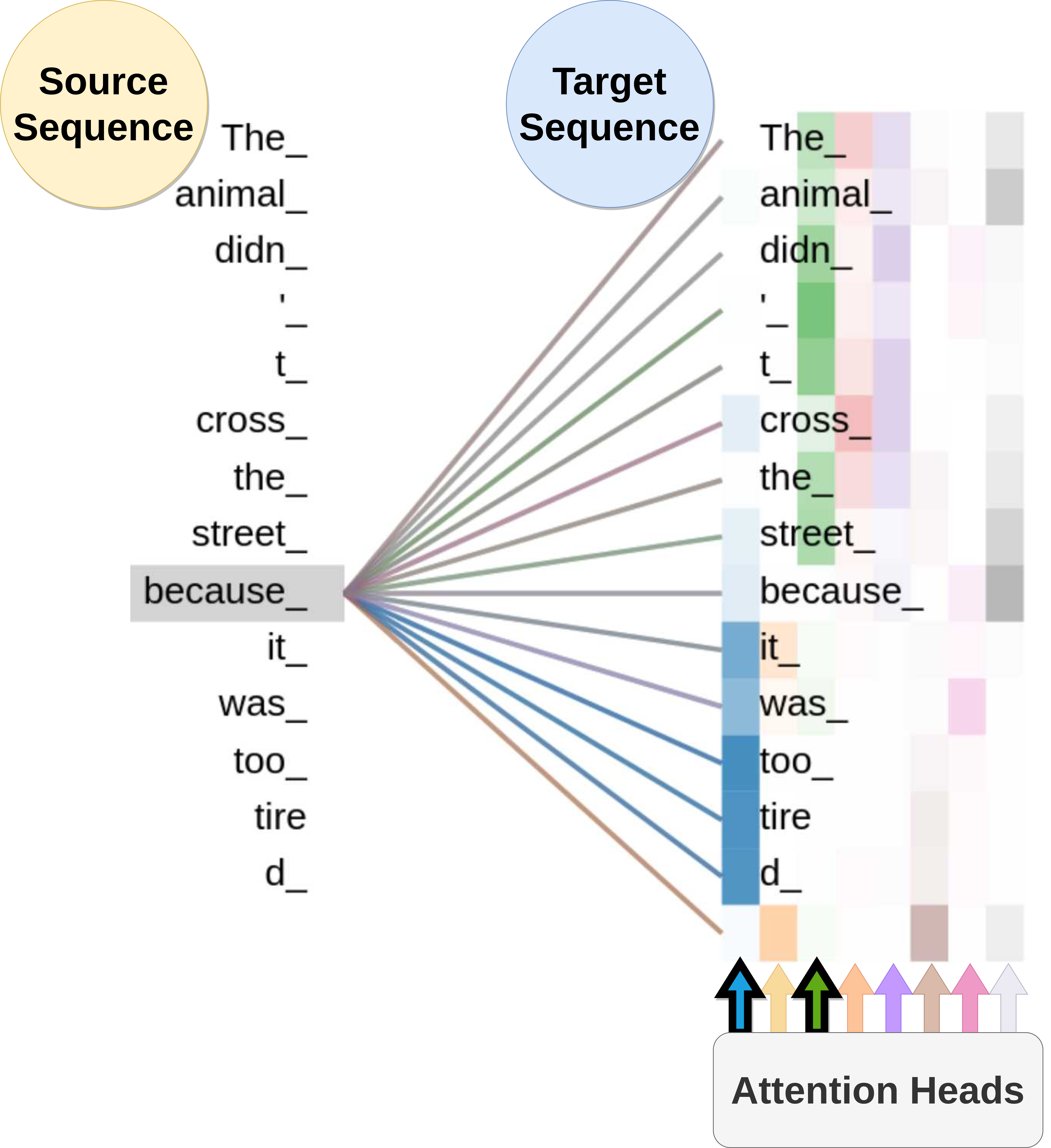
Figure 7: Matrix of alignment scores of the multi-head self attention model for the word «because» in the sentence «The animal didn’t cross the street because it was too tired». The image was produced using the pretrained Transformer via Tensor2tensor (Vaswani et al., 2018).
The scaled dot product attention is used in all instances of the attention mechanism in the Transformer model, since it can be implemented using highly optimized matrix multiplication algorithms. Transformer views the encoded representation as key-value pairs \((K,V)\) of dimension \(n\), although both the keys and values are the encoder hidden states, this distinction in notation helps with better understanding of the model. The output of the decoder is represented by \(Q\), the query, of size \(m\). The attention is defined as:
\[\mathrm{Attention}(Q,K,V) = \mathrm{softmax}\left( \frac{QK^T}{\sqrt{n}}\right)V\]The multi-head attention with \(h\) heads performs the above operation \(h\) times, then concatenates the outputs and performs a linear transformation for the final result, given as:
\[\begin{aligned} \mathrm{MultiHead}(Q, K, V ) &= [\mathrm{head}_1,\dots, \mathrm{head}_h]W^O \\ \text{where} \hspace{0.2cm} \mathrm{head}_i &= \mathrm{Attention}(QW_i^Q,KW_i^K,VW_i^V) \end{aligned}\]Where \(W^O\), \(W_i^Q\), \(W_i^K\), and \(W_i^V\) are matrix projections to be learned. Figure 8 shows the multi-head attention architecture.
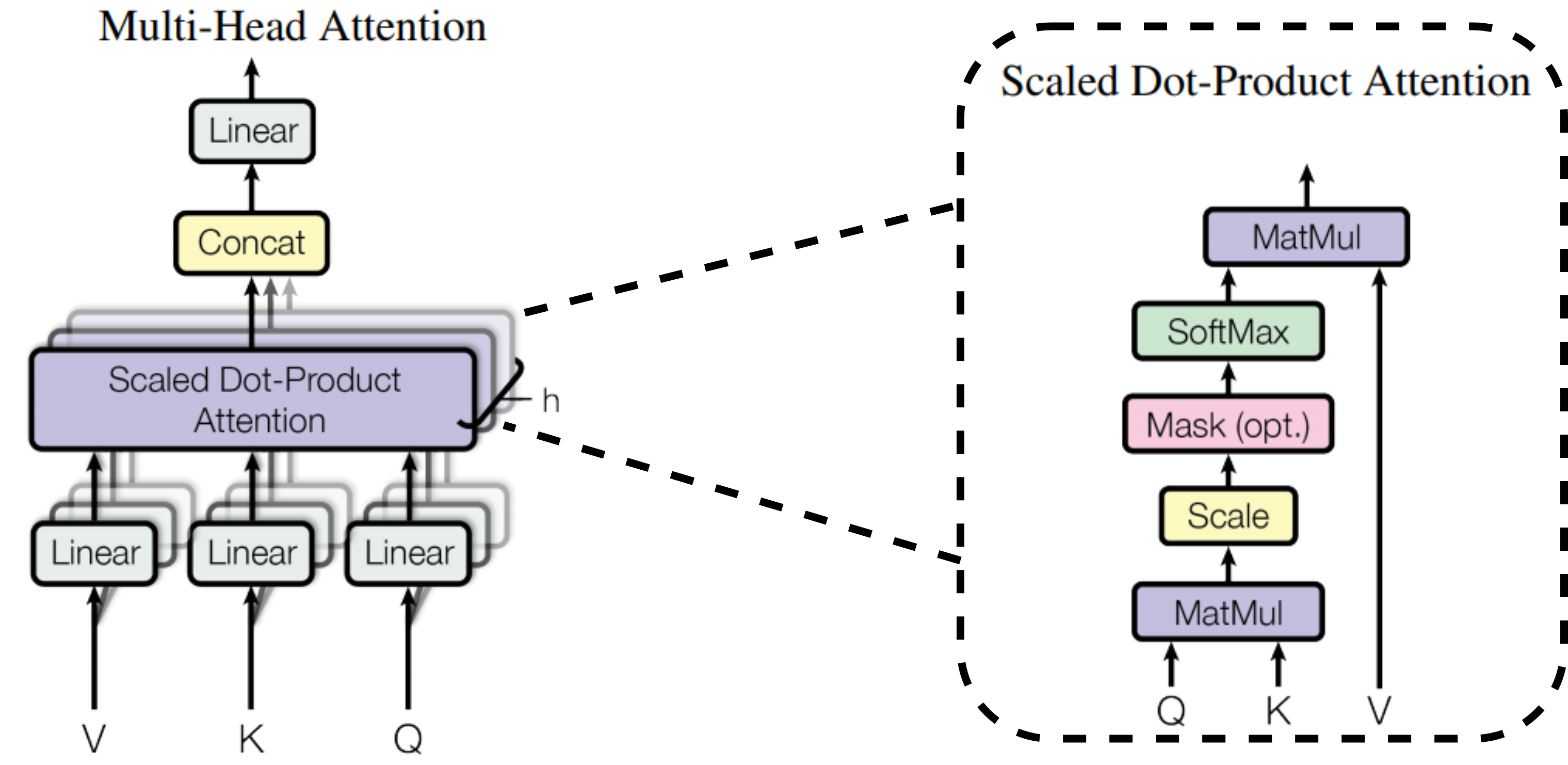
Figure 8: Multi-head attention architecture. The image was taken from (Vaswani et al., January 2017).
Model Architecture
The Transformer model was developed specifically for the NMT and follows the same principles of the sequence to sequence models (Sutskever et al., December 2014). The model is comprised of two modules: the encoder and the decoder module.
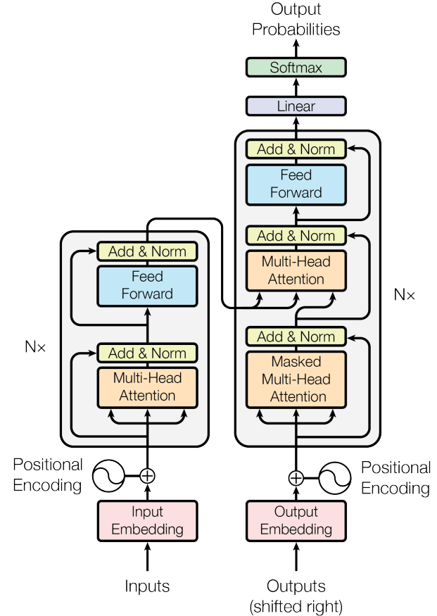
Figure 9: Transformer model architecture. The image was taken from (Vaswani et al., January 2017).
The encoder module (shown on the left side of Figure 9 generates an attention-based representation. It consists of a stack of 6 identical layers, where each layer is composed of 2 sublayers: a multi-head attention layer, and a position-wise fully connected feed-forward network. In order to encourage gradient flow in each sublayer, a residual connection (He et al., June 2016) is formed followed by a normalization layer (Ba et al., July 2016), i.e. the output of each sublayer is given by:
\[\mathrm{Output} = \mathrm{LayerNorm}\left(x + \mathrm{Sublayer}(x)\right)\]Where \(\mathrm{Sublayer}(x)\) is the function implemented by the sublayer itself.
The decoder module (see the right side of Figure 9) also consists of a stack of 6 identical layers. Similar to the encoder, each layer is composed of sublayers. In addition to the two sublayers in each encoder layer, the decoder incorporates a third sublayer, which performs multi-head attention over the output of the encoder stack. Analogous to the encoder module, each sublayer adopts a residual connection, and a layer normalization. The first multi-head attention sublayer of the decoder module is modified with a masking mechanism, in order to prevent the decoder to look into the future.
The Transformer model does not contain any recurrence or convolution, hence the model is unaware of the order of the sequence. In order to augment the model with this information a positional encoding is added to the input embeddings. The positional encoding captures the relative positioning of the elements of the sequence via \(\mathrm{sine}\) and \(\mathrm{cosine}\) functions of different frequencies. The \(i^{th}\) dimension of a positional encoding of size \(n\) for the \(j^{th}\) position is defined as:
\[\begin{aligned} \mathrm{Positional Encoding}_{(j, 2i)} &= \sin \left( \frac{j}{10000^{\frac{2i}{n}}} \right)\\ \mathrm{Positional Encoding}_{(j, 2i+1)} &= \cos \left( \frac{j}{10000^{\frac{2i}{n}}} \right) \end{aligned}\]Cite as:
@phdthesis{davari2020neural,
  title   = {Neural Network Approaches to Medical Toponym Recognition},
  author  = {Davari, MohammadReza},
  year    = {2020},
  month   = {April},
  school  = {Concordia University},
}
References
[1] Ba, J.L., Kiros, J.R., Hinton, G.E.: “Layer normalization”. arXiv preprint arXiv:1607.06450 (2016).
[2] Bahdanau, D., Cho, K., Bengio, Y.: “Neural machine translation by jointly learning to align and translate”. ICLR 2015.
[3] Bengio, Y., Simard, P., Frasconi, P., et al.: “Learning long-term dependencies with gradient descent is difficult”. TNNLS 1994.
[4] Britz, D., Goldie, A., Luong, M.T., Le, Q.: “Massive exploration of neural machine translation architectures”. EMNLP 2017.
[5] Cho, K., Van Merri enboer, B., Gulcehre, C., Bahdanau, D., Bougares, F., Schwenk,H., Bengio, Y.: “Learning phrase representations using rnn encoder-decoder for statistical machine translation”. EMNLP 2014.
[6] Devlin, J., Chang, M.W., Lee, K., Toutanova, K.: “BERT: Pre-training of deep bidirectional transformers for language understanding”. NAACL-HLT 2019.
[7] Graves, A., Wayne, G., Danihelka, I.: “Neural turing machines”. arXiv preprint arXiv:1410.5401 (2014).
[8] He, K., Zhang, X., Ren, S., Sun, J.: “Deep residual learning for image recognition”. CVPR 2016.
[9] Hoffman, J.E., Subramaniam, B.: “The role of visual attention in saccadic eye movements”. Perception & psychophysics (1995).
[10] Luong, T., Pham, H., Manning, C.D.: “Effective approaches to attention-based neural machine translation”. EMNLP 2015.
[11] Sutskever, I., Vinyals, O., Le, Q.V.: “Sequence to sequence learning with neural networks”. NIPS 2014.
[12] Vaswani, A., Shazeer, N., Parmar, N., Uszkoreit, J., Jones, L., Gomez, A.N., Kaiser, L., Polosukhin, I.: “Attention is all you need”. NIPS 2017.
[13] Vinyals, O., Kaiser, L., Koo, T., Petrov, S., Sutskever, I., Hinton, G.: “Grammar as a foreign language”. NIPS 2015.
[14] Xu, K., Ba, J., Kiros, R., Cho, K., Courville, A., Salakhudinov, R., Zemel, R.,Bengio, Y.: “Show, attend and tell: Neural image caption generation with visual attention”. ICML 2015.
[15] Yang, Z., Dai, Z., Yang, Y., Carbonell, J., Salakhutdinov, R.R., Le, Q.V.: “XLNet:Generalized autoregressive pretraining for language understanding”. NIPS 2019.